An Annotated Guide to PPO (Proximal Policy Optimization)

Introduction

I have written this article to explore my own intuition behind why the PPO algorithm works, and why is it preferred over other learning methods. This article by no means has mathematical depth or intuition that you would expect from a book or a series of lectures. My aim with this article is to explore some of the interesting things I have found out while implementing this algorithm from scratch and it’s various characteristics.

Off-Policy vs On-Policy

With that said, let’s begin exploring the main difference between off-policy and on-policy algorithms in RL, you might have heard mentioned in a lot of places but what exactly does it mean to say that an algorithm is “On-Policy”?

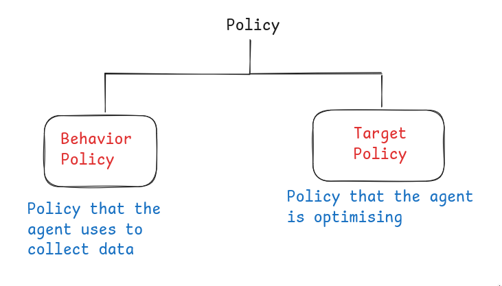
There are two types of Policy, behavior policy and target policy. Behavior policy is the one that the agent is using to collect data, and target policy is the one that agent updates.

When we say that an algorithm is On-Policy, it means that our agent is trying to optimize the same policy which it is using to collect data.

While Off-Policy means that the agent is trying to optimize a different policy than the one it is using to collect data.

Let’s take the example of SARSA algorithm. SARSA is an On-Policy algorithm because

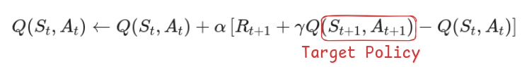Here the target policy is the same as the policy you are using to sample actions from, this makes it on-policy.

This algorithm requires data to be constantly generated and used. We cannot store data in a buffer and use that later on because that would break the On-Policy rule.

Here is the example of DQN (Which as in Off-Policy algorithm)

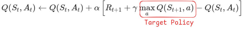
This algorithm is Off-Policy because we are following a greedy approach while sampling the target which is different than our behavior policy of epsilon-greedy. Here we can store data in a buffer and train our algorithm on old data as well.

Why use On-Policy algorithm?

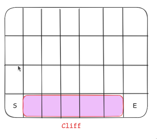
Let’s understand it through the cliff walking example. An agent is at the start of the grid denoted by S. Agent has to go to the end marked by E but the agent cannot fall into the cliff.

As for the rewards, the agent gets -1 for every step taken and -100 if it falls off the cliff.

So what do you think the path of the agent will look like if he followed an On-Policy algorithm vs Off-Policy?

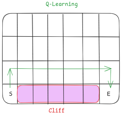
An Off-Policy algorithm like Q-Learning will give a path that is very close to the cliff, it will give a risky path because our target policy is so greedy that even if it gets a reward of -100 from falling off, it will still consider the path that is near to the cliff as safe.

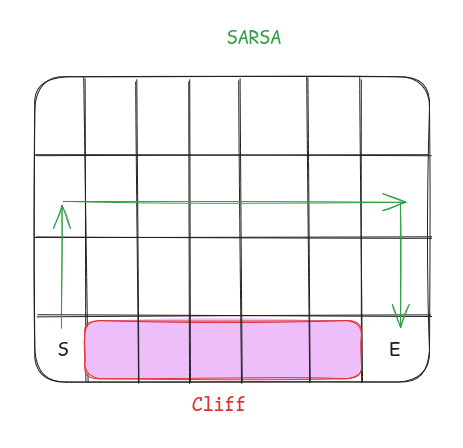
Whereas something like SARSA would prefer a path that is safe because the agent is trying to execute the same policy it learns. The agent will sometimes try to execute it’s own policy and fall off the cliff which the agent will be discouraged to do.

Here we would want our algorithm to behave more like SARSA because we don’t want our agent to become unstable and have a risk of falling down the cliff.

The PPO algorithm

Now let’s go through the code implementation of the PPO algorithm and see how it works. PPO is an on-policy algorithm that is used extensively in Robotics.

For this we are going to solve the Pendulum V1 environment by OpenAI gym.

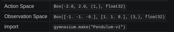
Here our action space is going to have a dimension of 1 as it is just the torque applied to free end of the pendulum. Observation space is x,y,w which denotes the Cartesian coordinates and angular velocity of the free end, this is of dimension 3.

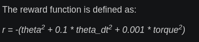
This is the reward function

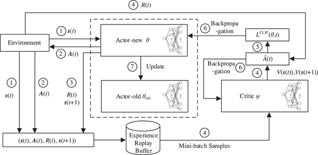
This is the architecture we are going to code and implement. For now just take an overview and we will uncover the details later.

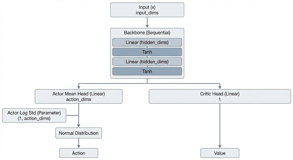
Let’s define the brain of our agent first. We want our agent to have two heads, an actor and a critic, the actor is supposed to output the probability distribution of the action and the critic is supposed to output the value of the current state we are in.

Our goal with the agent is that it should be able to output a normal distribution for the action. We want a distribution instead of a single value because our action space is continuous and it should be able to sample from that distribution.

As for the critic, we just want a single value that estimates the value of the state that the agent is currently in.

Both the heads will share the same backbone here and that can be a simple multi layer perceptron.

Other small things to keep in mind is that in PPO, when we want to evaluate steps from an old policy then we often use something called a ratio. In order to compute ratio, we require the log probability of the old action. We also want the total entropy of our action as we will be using it as a loss to help PPO explore more.

With all this in mind, can you design the PPO agent?

src/agent.py

import torch
import torch.nn as nn
import torch.distributions as distributions
import numpy as np
from src.utils import layer_init
 
class PPO(nn.Module):
    def __init__(self, input_dims, hidden_dims, action_dims, lr=3e-4):
        super().__init__()
 
        self.backbone = nn.Sequential(
            layer_init(nn.Linear(input_dims, hidden_dims)),
            nn.Tanh(),
            layer_init(nn.Linear(hidden_dims, hidden_dims)),
            nn.Tanh()
        )
 
        self.actor_mean = layer_init(nn.Linear(hidden_dims, action_dims), 
        std=0.01)
        
        self.actor_log_std = nn.Parameter(torch.zeros(1, action_dims))
 
        self.critic_head = layer_init((nn.Linear(hidden_dims, 1)), std = 1)
    
    def get_value(self, x):
        features = self.backbone(x)
        value = self.critic_head(features)
 
        return value.reshape(-1)
    
    def get_action_and_value(self, x, action = None):
        features = self.backbone(x)
 
        mean = self.actor_mean(features)
        std = self.actor_log_std.exp()
 
        dist = distributions.Normal(mean, std)
 
        if action is None:
            action = dist.sample()
 
        value = self.critic_head(features)
 
        return action, dist.log_prob(action).sum(1), dist.entropy().sum(1), 
        value.reshape(-1)

Experience Replay Buffer

Now, in PPO we would also have a replay buffer, an agent will collect a certain number of transitions and we would want to use those transitions for a certain number of epochs (around 5-10) to squeeze more information out of it, and then we will throw this information out. This is better than actor critic methods as we are able to squeeze out more information out of the same buffer. We will see why this works later on and what trick does PPO use in order to do this.

In this replay buffer we mainly want to store states, actions, rewards, log_probs, values and dones. We want to store these values mainly because of the GAE (Generalized Advantage Estimate)

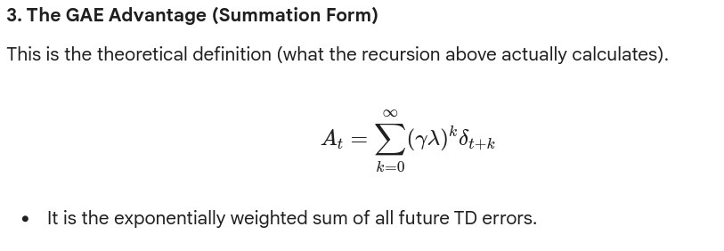
GAE (Generalized Advantage Estimate)

Let’s see the equations to understand GAE

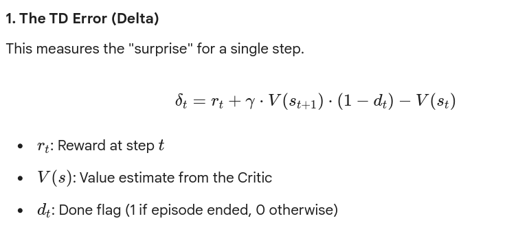
So, at every step, we compute a value delta, we can also call it “surprise” (this is not an official term, just a term that I think is suitable). The surprise tells how much the value of this state deviates from the agent’s estimate if we just look at the next state.

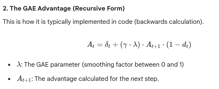
Then if we intuitively think about advantage (At), then advantage is just the discounted sum of all the surprises.

Let’s understand this through a numerical example

This example below was generated by Gemini to understand what would happen if we just used One-Step TD vs Monte-Carlo Bootstrapping vs GAE

Here is the step-by-step mathematical breakdown of the “Gold Mine” example.

The Setup

• Trajectory: $S_1\stackrel{r_1}{\to }{S}_2\stackrel{r_2}{\to }{S}_3\stackrel{r_3}{\to }\text{End}$

• Rewards:

  • $r_1=0$ (Step 1)

  • $r_2=0$ (Step 2)

  • $r_3=100$ (Step 3 - The Gold Mine)

• Current Value Estimates (The Dumb Critic):

  • $V(S_1)=10$

  • $V(S_2)=10$

  • $V(S_3)=10$

  • $V(\text{End})=0$

• Discount Factor: $\gamma =0.9$

We want to calculate the Target Value for State 1 ($V_{target}(S_1)$). This is what we will tell the network $S_1$ should have been.

---

Method 1: One-Step TD (TD Error only)

Corresponds to gae_lambda = 0.

This method only looks at the immediate reward and the estimated value of the very next state. It ignores everything after $S_2$.

$V_{target}(S_1)=r_1+\gamma \cdot V(S_2)$

$V_{target}(S_1)=0+0.9\cdot 10$

$V_{target}(S_1)=9$

Result: The target is 9.

• Intuition: The agent failed to see the Gold Mine. It blindly trusted that $S_2$ is worth 10, so it updated $S_1$ to be slightly less than 10 (due to discounting).

---

Method 2: Monte Carlo

Corresponds to gae_lambda = 1.

This method sums up the actual discounted rewards received until the end of the episode. It ignores the Value function entirely (except for bootstrapping at the very end if the episode wasn’t done, but here it is done).

$V_{target}(S_1)=G_1=r_1+\gamma r_2+{\gamma }^2{r}_3$

$V_{target}(S_1)=0+(0.9\cdot 0)+(0.9^2\cdot 100)$

$V_{target}(S_1)=0+0+(0.81\cdot 100)$

$V_{target}(S_1)=81$

Result: The target is 81.

• Intuition: The agent saw the Gold Mine perfectly. It ignored its own bad predictions ($V(S_2)$) and trusted the raw reality.

---

Method 3: Generalized Advantage Estimation (GAE)

Corresponds to gae_lambda = 0.5 (for this example).

This is the hybrid. First, we must calculate the “local errors” ($\delta$) for every step in the chain.

Step A: Calculate the local TD Errors ($\delta$)

The formula is: ${\delta }_t=r_t+\gamma V(S_{t+1})-V(S_t)$

1. For Step 1:

   ${\delta }_1=0+0.9(10)-10=-1$

   (Prediction was slightly too high compared to neighbor)

2. For Step 2:

   ${\delta }_2=0+0.9(10)-10=-1$

   (Prediction was slightly too high compared to neighbor)

3. For Step 3:

   ${\delta }_3=100+0.9(0)-10=90$

   (MASSIVE surprise! We expected 10, got 100)

Step B: Calculate the Advantage ($A$) for State 1

We sum the errors, decaying them by $(\gamma \cdot \lambda )$ each step.

Let’s use $\lambda =0.5$.

Decay factor $(\gamma \lambda )=0.9\times 0.5=0.45$.

$A^{GAE}(S_1)={\delta }_1+(\gamma \lambda ){\delta }_2+(\gamma \lambda {)}^2{\delta }_3$

$A^{GAE}(S_1)=-1+(0.45\cdot -1)+(0.45^2\cdot 90)$

$A^{GAE}(S_1)=-1-0.45+(0.2025\cdot 90)$

$A^{GAE}(S_1)=-1.45+18.225$

$A^{GAE}(S_1)\approx 16.77$

Step C: Calculate the Target

Target = Old Estimate + Advantage

$V_{target}(S_1)=V(S_1)+A^{GAE}(S_1)$

$V_{target}(S_1)=10+16.77$

$V_{target}(S_1)=26.77$

---

Comparison of Results

Method	Target for S1​	What happened?
TD (One-Step)	9	It barely moved. It didn’t see the gold mine at all.
Monte Carlo	81	It moved all the way to reality. Maximum variance.
GAE ($\lambda =0.5$)	26.77	It saw the gold mine (${\delta }_3=90$), but by the time that information traveled back to $S_1$, it was dampened. It moved the value up significantly (from 10 to 26), but not recklessly.

By adjusting $\lambda$, you control how much of that “90” surprise at the end is allowed to flow back to the start.

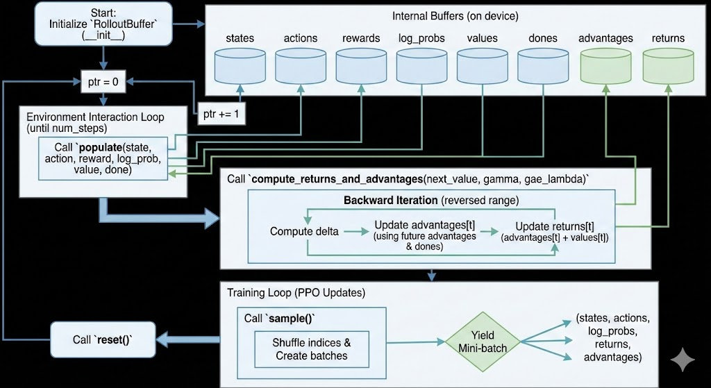
Now let’s talk about the design of our replay buffer. We want our replay buffer to populate state, actions, rewards, values etc. We also want to sample from it and we also want to make the computing of GAE a part of the replay buffer.

So can you design a buffer that satisfies these constraints?

src/buffer.py

import torch
 
class RolloutBuffer():
    def __init__(self, num_steps, state_dim, action_dim, batch_size, 
    device='cuda'):
        self.states = torch.zeros((num_steps, state_dim), device = device)
        self.actions = torch.zeros((num_steps, action_dim), device=device)
        self.rewards = torch.zeros(num_steps, device=device)
        self.log_probs = torch.zeros(num_steps, device=device)
        self.values = torch.zeros(num_steps, device=device)
        self.dones = torch.zeros(num_steps, device=device)
 
        self.advantages = torch.zeros(num_steps, device=device)
        self.returns = torch.zeros(num_steps, device=device)
 
        self.num_steps = num_steps
        self.batch_size = batch_size
        self.ptr = 0
 
    def populate(self, state, action, reward, log_prob, value, done):
        self.states[self.ptr] = state
        self.actions[self.ptr] = action
        self.rewards[self.ptr] = reward
        self.log_probs[self.ptr] = log_prob
        self.values[self.ptr] = value
        self.dones[self.ptr] = done
 
        self.ptr += 1
 
    def reset(self):
        self.ptr = 0
        
    def sample(self):
        indices = torch.randperm(self.num_steps)
 
        for start in range(0, self.num_steps, self.batch_size):
            end = start + self.batch_size
            batch_indices = indices[start:end]
 
            yield (
                self.states[batch_indices],
                self.actions[batch_indices],
                self.log_probs[batch_indices],
                self.returns[batch_indices],
                self.advantages[batch_indices]
            )
 
    def compute_returns_and_advantages(self, next_value, gamma=0.99, 
    gae_lambda=0.95):
        for t in reversed(range(len(self.advantages))):
            if t == len(self.advantages) - 1:
                delta = self.rewards[t] + gamma*next_value*(1 - self.dones[t]) - 
                self.values[t]
                
                self.advantages[t] = delta
                self.returns[t] = self.advantages[t] + self.values[t]
            else:
                delta = self.rewards[t] + gamma*self.values[t + 1]*(1 - 
                self.dones[t]) - self.values[t]
                
                self.advantages[t] = delta + gamma*gae_lambda*self.advantages[t 
                + 1]*(1 - self.dones[t])
                  
                self.returns[t] = self.advantages[t] + self.values[t]

Trainer

Now we come to the main part of the algorithm, this is where PPO differentiates itself from other algorithms, it introduces some clever tricks that makes PPO better than other On-Policy algorithms.

The first trick is regarding the reuse of steps in the buffer. In a normal On-Policy algorithm you cannot reuse the steps but PPO introduces something called ratio which allows us to be more sample efficient by re-using data generated from a slightly older policy to train our agent.

Let us understand the equations

1. The Probability Ratio ($r_t(\theta )$)

This measures “how much has the policy changed” for a specific action $a_t$ in state $s_t$ since we collected the data.

The Equation:

$r_t(\theta )=\frac{{\pi }_{\theta }(a_t|s_t)}{{\pi }_{{\theta }_{old}}(a_t|s_t)}$

• ${\pi }_{\theta }$: The probability of taking action $a_t$ under the current updated network.

• ${\pi }_{{\theta }_{old}}$: The probability of taking action $a_t$ under the old network (the one that played the game).

In Code (The Log Trick):

Computers hate multiplying tiny probabilities (floating point underflow), so we work in logs.

$r_t(\theta )=\exp (\log {\pi }_{\theta }-\log {\pi }_{{\theta }_{old}})$

Intuition:

• $r_t>1$: The action is more likely now than before.

• $r_t<1$: The action is less likely now than before.

• $r_t=1$: The policy hasn’t changed.

---

2. The Clipped Surrogate Objective ($L^{CLIP}$)

This is the most famous part of PPO. It tries to maximize rewards while ensuring the new policy doesn’t wander too far from the old one.

The Equation:

$L^{CLIP}(\theta )={\hat{\mathbb{E}}}_t\left[\min \left(r_t(\theta ){\hat{A}}_t,\text{clip}(r_t(\theta ),1-ϵ,1+ϵ){\hat{A}}_t\right)\right]$

Let’s break this down into two cases based on the Advantage (${\hat{A}}_t$).

Case A: The Action was Good (${\hat{A}}_t>0$)

The action resulted in better-than-expected rewards. We want to increase its probability ($r_t>1$).

• Unclipped Term ($r_t{\hat{A}}_t$): Encourages raising $r_t$ infinitely.

• Clipped Term: Caps $r_t$ at $1+ϵ$ (usually $1.2$).

• The Logic: If the probability increases by more than 20%, the min operator selects the clipped version. The gradient becomes 0, and the update stops.

  • Result: “Increase the probability, but don’t get too greedy.”

Case B: The Action was Bad (${\hat{A}}_t<0$)

The action resulted in poor rewards. We want to decrease its probability ($r_t<1$).

• Unclipped Term: Encourages lowering $r_t$ to 0.

• Clipped Term: Caps $r_t$ at $1-ϵ$ (usually $0.8$).

• The Logic: If the probability decreases by more than 20%, the min (which acts like a max for negative numbers) selects the clipped version. The update stops.

  • Result: “Decrease the probability, but don’t destroy the policy completely.”

---

3. The Critic Loss ($L^{VF}$)

The Critic’s only job is to accurately predict the “True Return” ($R_t$). This is a standard regression problem.

The Equation:

$L_t^{VF}=(V_{\theta }(s_t)-R_t{)}^2$

• $V_{\theta }(s_t)$: The value predicted by the neural network right now.

• $R_t$: The target return calculated using GAE ($Returns=Advantage+V_{old}$).

The Total Critic Loss:

We average this over the entire batch:

$L^{VF}=\frac{1}{N}{\sum }_{i=1}^N(V_{\theta }(s_i)-R_i{)}^2$

Why use MSE?

By minimizing the Mean Squared Error (MSE), the Critic network learns to output the expected sum of discounted rewards, which helps reduce the variance of the Actor’s updates in the future.

---

Summary of the “Loss” Direction

In standard optimization (like SGD or Adam), we minimize a loss. PPO is designed to maximize an objective.

To fix this, the final code equation flips the signs for the Actor:

$Loss=\underset{\text{Make negative to minimize}}{\underbrace{-L^{CLIP}}}+\underset{\text{Already a loss (MSE)}}{\underbrace{0.5\cdot L^{VF}}}-\underset{\text{Subtract entropy}}{\underbrace{0.01\cdot S}}$

• Maximizing Objective $\to$ Minimizing Negative Objective.

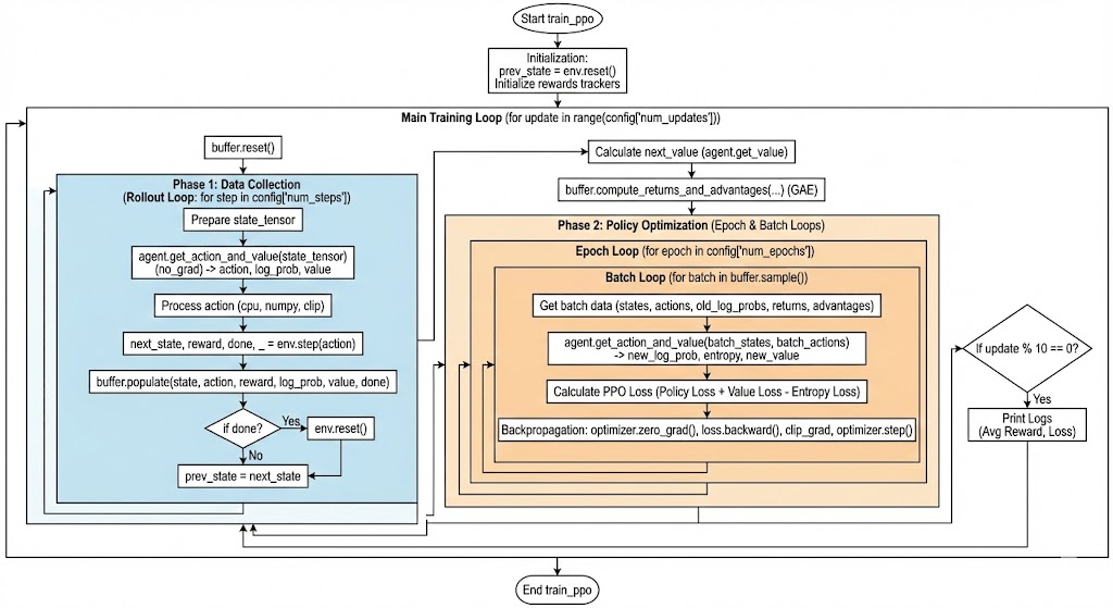
So now we want a trainer that performs steps in the environment, stores them in the replay buffer, computes the GAE, iterates over the data for certain number of epochs, minimizes the loss, and then repeats the process again.

Can you design a trainer that does this?

src/trainer.py

import torch
import torch.nn as nn
import numpy as np
 
def train_ppo(env, agent, buffer, optimizer, config):
    device = config['device']
    prev_state, _ = env.reset()
    
    episode_rewards = []
    current_ep_reward = 0
 
    for update in range(config['num_updates']):
        buffer.reset()
        
        for step in range(config['num_steps']):
            state_tensor = torch.as_tensor(prev_state, dtype=torch.float32, 
            device=device)
            state_tensor = state_tensor.reshape(1, -1)
            
            with torch.no_grad():
                action, log_prob, _, value = 
                agent.get_action_and_value(state_tensor)
 
            action_numpy = action.cpu().numpy()
            clipped_action = np.clip(action_numpy, -2, 2).flatten()
            
            next_state, reward, terminated, truncated, _ = 
            env.step(clipped_action)
            
            done = terminated or truncated
            
            if isinstance(reward, np.ndarray):
                reward = reward.item()
            
            current_ep_reward += reward
 
            buffer.populate(
                state_tensor, action, 
                torch.as_tensor(reward, dtype=torch.float32, device=device),
                log_prob, value, 
                torch.as_tensor(int(done), dtype=torch.float32, device=device)
            )
 
            prev_state = next_state
            if done:
                prev_state, _ = env.reset()
                episode_rewards.append(current_ep_reward)
                current_ep_reward = 0
 
        with torch.no_grad():
            next_state_tensor = torch.as_tensor(prev_state, dtype=torch.float32, 
            device=device)
            
            next_state_tensor = next_state_tensor.reshape(1, -1)
            next_value = agent.get_value(next_state_tensor)
        
        buffer.compute_returns_and_advantages(
            next_value, config['gamma'], config['gae_lambda']
        )
 
        b_v_losses = []
        
        for epoch in range(config['num_epochs']):
            for batch in buffer.sample():
                b_states, b_actions, b_log_probs, b_returns, b_advantages = batch
            
                _, new_log_prob, entropy, new_value = 
                agent.get_action_and_value(b_states, action=b_actions)
                
                log_ratio = new_log_prob - b_log_probs
                ratio = log_ratio.exp()
 
                b_advantages = (b_advantages - b_advantages.mean()) / 
                (b_advantages.std() + 1e-8)
 
                pg_loss1 = -b_advantages * ratio
                pg_loss2 = -b_advantages * torch.clamp(ratio, 1 - 0.2, 1 + 0.2)
                pg_loss = torch.max(pg_loss1, pg_loss2).mean()
 
                v_loss = 0.5 * ((new_value - b_returns) ** 2).mean()
                entropy_loss = entropy.mean()
 
                loss = pg_loss + v_loss * 0.5 - entropy_loss * 0.01
 
                optimizer.zero_grad()
                loss.backward()
                nn.utils.clip_grad_norm_(agent.parameters(), 0.5)
                optimizer.step()
                
                b_v_losses.append(v_loss.item())
 
        if (update + 1) % 10 == 0:
            avg_reward = np.mean(episode_rewards[-10:]) if episode_rewards else 
            0.0
            
            print(f"Update {update+1}/{config['num_updates']} | Avg Reward: 
            {avg_reward:.2f} | Value Loss: {np.mean(b_v_losses):.4f}")

Main Loop

Now we just have to define hyper-parameters and train our PPO agent

main.py

import gymnasium as gym
import torch
import torch.optim as optim
 
from src.agent import PPO
from src.buffer import RolloutBuffer
from src.trainer import train_ppo
from src.utils import get_device, seed_everything
 
def main():
    config = {
        "model_id": "model-v1",
        "env_id": "Pendulum-v1",
        "total_steps": 1_000_000,
        "num_steps": 2048,     
        "batch_size": 64,
        "num_epochs": 10,
        "hidden_dims": 64,
        "learning_rate": 3e-4,
        "gamma": 0.99,
        "gae_lambda": 0.95,
        "seed": 42,
    }
    
    config["num_updates"] = int(config["total_steps"] / config["num_steps"])
    config["device"] = get_device()
    
    print(f"Running PPO on {config['env_id']} using {config['device']}")
    
    seed_everything(config["seed"])
    env = gym.make(config["env_id"])
    
    action_dim = env.action_space.shape[0]
    state_dim = env.observation_space.shape[0]
    
    agent = PPO(state_dim, config["hidden_dims"], 
    action_dim).to(config["device"])
    
    buffer = RolloutBuffer(
        config["num_steps"], 
        state_dim, 
        action_dim, 
        config["batch_size"], 
        device=config["device"]
    )
    
    optimizer = optim.Adam(agent.parameters(), lr=config["learning_rate"], 
    eps=1e-5)
    
    train_ppo(env, agent, buffer, optimizer, config)
 
    save_path = f"ppo_{config['model_id']}.pth"
    torch.save(agent.state_dict(), save_path)
    print(f"Model saved to {save_path}")
    
    env.close()
 
if __name__ == "__main__":
    main()

That’s about it for this PPO implementation. Thanks for reading